Notes on python's pandas and performance

For data analysis, I sometimes use python in combination with pandas. In this post I’ll take a look at some of the performance aspects of pandas and alternatives. Pandas makes it easy to read data using read_csv (or other read_ functions). You get a DataFrame which is easy to query and plot using matplotlib.

Other manipulations are also possible, for example here’s a simple string-split into some seperate columns:

1
2
3
4

data_original = pd.read_csv('httplogs.csv')
# Request looks like so: "GET /973585cf-3619-4fca-b218-7dbf5b27ef61/login HTTP/1.1"
data_original["HTTPMethod"] = data_original["request"].str.split(" ").str[0]
data_original["TenantID"] = data_original["request"].str.split("/").str[1]

This analysis and manipulation can also be done in tools like Excel. My expirience is that I can combine the retrieval of data, parsing and analysis in one jupyter notebook. I also find excel too fragile and too manual when you start working with multiple files or a few different manipulations. Don’t get me wrong, I think Excel is a great tool, but I’ve never liked how it works when doing data processing like this. Learning python took time. It’s a great language but in the beginning my work took longer than in Excel, and the tradeoff between automating things in python was difficult. Now that I know python and pandas better, I realize that I’m sometimes faster and end up with solutions that are less error-prone and more repeatable.

More complex data

Above example does a simple pd.read_csv('httplogs.csv'). There are other read_ functions in python that can deal with other data types, and you can also tell read_csv how you want data to be parsed. Here’s an example of parsing HTTP logfiles (which are technically not CSV files):

1
2
3
4
5
6
7
8
9

# Read without converters
pd.read_csv(
    'vhostcombined.log',
    sep=r'\s(?=(?:[^"]*"[^"]*")*[^"]*$)',
    engine='python',
    na_values='-',
    header=None,
    usecols=[0, 2, 4, 5, 7, 8, 9, 10, 11],
    names=['vhost', 'ip', 'user', 'time', 'request', 'status', 'size', 'referer', 'user_agent'])

Parsing data on read

The above example read_csv code produces the following dataframe:

RangeIndex: 94047 entries, 0 to 94046
Data columns (total 9 columns):
 #   Column      Non-Null Count  Dtype 
---  ------      --------------  ----- 
 0   vhost       94010 non-null  object
 1   ip          94047 non-null  object
 2   user        8209 non-null   object
 3   time        94047 non-null  object
 4   request     94047 non-null  object
 5   status      94047 non-null  int64 
 6   size        94047 non-null  int64 
 7   referer     94047 non-null  object
 8   user_agent  94047 non-null  object
dtypes: int64(2), object(7)
memory usage: 6.5+ MB

Note that the time is an object. Normally we’d do something like data_original["time"] = pd.to_datetime(data_original["time"], utc=True) to convert this, but in my case the seperator code and logfile produces a time with [] around it. That’s just how my logfile is generated by the HTTP server. We also have some other string issues to deal with.

The following resolves that for me:

 1
 2
 3
 4
 5
 6
 7
 8
 9
10
11
12
13
14
15
16
17

# Read with converters
def parse_str(x):
    return x[1:-1]

def parse_datetime(x):
    dt = datetime.strptime(x[1:], '%d/%b/%Y:%H:%M:%S')
    return dt

data_original = pd.read_csv('vhostcombined.log',
    sep=r'\s(?=(?:[^"]*"[^"]*")*[^"]*$)', engine='python', na_values='-', header=None, usecols=[0, 2, 4, 5, 7, 8, 9, 10, 11],
    names=['vhost', 'ip', 'user', 'time', 'request', 'status', 'size', 'referer', 'user_agent'],
    converters={'time': parse_datetime,
                'status': int,
                'size': int,
                'request': parse_str,
                'referer': parse_str,
                'user_agent': parse_str})

This code was copied/inspired by this handy post by Modesto Mas.

Performance

Over time, data grows and this means that you can end up parsing milions of lines of CSV quite quickly. I started noticing that some of my python became slow and I started looking at performance.

My primary performance questions are:

• How can i speed up reading data, primarily when i have a few manipulations like the parse_datetime and parse_str
• How can selections (DataFrame.loc[]) and groupby’s within the data be speed up, as I probably want to plot() the result

To check out some of the performance, I used the great magic function %timeit to compare the two ways of reading the HTTP logfile.

Read with converters: 1.87 s ± 16.1 ms per loop (mean ± std. dev. of 5 runs, 5 loops each)
Read without converters: 1.11 s ± 70.8 ms per loop (mean ± std. dev. of 5 runs, 5 loops each)

Everybody expected the additional parsing to slow things down - no suprise there. What if we used the read_csv without the converters and applied a .apply() like so:

1
2
3
4
5
6
7
8
9

# Using .apply() to perform data transformation
data_original = pd.read_csv('vhostcombined.log',
    sep=r'\s(?=(?:[^"]*"[^"]*")*[^"]*$)', engine='python', na_values='-', header=None, usecols=[0, 2, 4, 5, 7, 8, 9, 10, 11],
    names=['vhost', 'ip', 'user', 'time', 'request', 'status', 'size', 'referer', 'user_agent'])

data_original["time"] = data_original["time"].apply(parse_datetime)
data_original["request"] = data_original["request"].apply(parse_str)
data_original["referer"] = data_original["referer"].apply(parse_str)
data_original["user_agent"] = data_original["user_agent"].apply(parse_str)

Which results in:

1.95 s ± 35 ms per loop (mean ± std. dev. of 5 runs, 5 loops each)

This is not faster then reading data with converters.

Swifter

Swifter is a library that can help speed up pandas performance. It’s super easy to use:

 1
 2
 3
 4
 5
 6
 7
 8
 9
10

# Using swifter.apply() to perform data transformation
data_original = pd.read_csv('vhostcombined.log',
    sep=r'\s(?=(?:[^"]*"[^"]*")*[^"]*$)', engine='python', na_values='-', header=None, usecols=[0, 2, 4, 5, 7, 8, 9, 10, 11],
    names=['vhost', 'ip', 'user', 'time', 'request', 'status', 'size', 'referer', 'user_agent'])


data_original["time"] = data_original["time"].swifter.apply(parse_datetime)
data_original["request"] = data_original["request"].swifter.apply(parse_str)
data_original["referer"] = data_original["referer"].swifter.apply(parse_str)
data_original["user_agent"] = data_original["user_agent"].swifter.apply(parse_str)

unfortunately, in this specific case it does not improve performance:

2.65 s ± 252 ms per loop (mean ± std. dev. of 5 runs, 5 loops each)

This is not an improvement. Where swifter does seem to shine is when data can be vectorized, and in the above example that’s not possible.

Dask

Dask is a library to help with parallel computing in python. You can also easily install it and there are useful functions to convert from a pandas DataFrame to a dask DataFrame. I rewrote the above code to use dask to read the data and perform the data manipulation. I was so impressed in the beginning, because i wasn’t aware of dask’s lazy evaluation. The .compute() actually performs the code and the end result looks like this:

 1
 2
 3
 4
 5
 6
 7
 8
 9
10
11
12

data_original = dd.read_csv('vhostcombined.log',
    sep=r'\s(?=(?:[^"]*"[^"]*")*[^"]*$)', engine='python', na_values='-', header=None, usecols=[0, 2, 4, 5, 7, 8, 9, 10, 11],
    names=['vhost', 'ip', 'user', 'time', 'request', 'status', 'size', 'referer', 'user_agent'],
    dtype={'user': object})

data_original["time"] = data_original["time"].apply(parse_datetime, meta=datetime)
data_original["request"] = data_original["request"].apply(parse_str, meta=str)
data_original["referer"] = data_original["referer"].apply(parse_str, meta=str)
data_original["user_agent"] = data_original["user_agent"].apply(parse_str, meta=str)

df = data_original.compute()

It results in:

1.82 s ± 82.5 ms per loop (mean ± std. dev. of 5 runs, 5 loops each)

The df variable above is a pandas dataframe, so we also spend some time on converting a dask dataframe to a pandas dataframe, but it is faster.

Polars

Polars is yet another python library. It’s based on rust. It’s a DataFrame library so it should be able to do what pandas is able to do as well, but is aimed on performance. This sounds great, and it does seem very fast. The downside is that the syntax of your code has to change quite a lot. You’re no longer writing “pandas code”, you’re writing “python using polars”. This is not a huge deal, but it does take some time to get used to.

Here’s an example of our code after changing it to polars *and still using the pandas read_csv():

 1
 2
 3
 4
 5
 6
 7
 8
 9
10

# Using Polars after converting from Pandas
tmpdf = pd.read_csv('vhostcombined.log', 
    sep=r'\s(?=(?:[^"]*"[^"]*")*[^"]*$)', engine='python', na_values='-', header=None, usecols=[0, 2, 4, 5, 7, 8, 9, 10, 11],
    names=['vhost', 'ip', 'user', 'time', 'request', 'status', 'size', 'referer', 'user_agent'])

data_original = pl.from_pandas(tmpdf)
data_original = data_original.with_columns(pl.col("time").apply(parse_datetime, pl.Datetime))
data_original = data_original.with_columns(pl.col("request").apply(parse_str, pl.Utf8))
data_original = data_original.with_columns(pl.col("referer").apply(parse_str, pl.Utf8))
data_original = data_original.with_columns(pl.col("user_agent").apply(parse_str, pl.Utf8))

It results in:

2 s ± 76.4 ms per loop (mean ± std. dev. of 5 runs, 5 loops each)

This time isn’t better than the original code. A whole new syntax is needed, and we had to learn about different data types (note the pl.Utf8). I also timed the pl.from_pandas(tmdf) as 29ms. This would mean that the .apply() are not specifically faster. It would likely be better if we could perform the read_csv within polars, but unfortunately their method doesn’t support the regular expression syntax. At this time it’s also good to point out that there might be some polar expressions that could do what the above code does, which might speed things up.

Reading data conclusion / Using the data

So far, we’ve just read a (not particularly massive) CSV into a dataframe and applied a few manipulations to it. We’ve found that there are alternative libraries that are aimed on performance, but we’re not nessasarily seeing the increase in speed at this stage.

Reading the data is only the start. Quite often I do it only once and then select, group and plot the data to analyse it. Let’s say i wanted to see a distribution of HTTP method for a specific vhost:

1
2
3
4

# Pandas plot()
data_original["HTTPMethod"] = data_original["request"].str.split(" ").str[0]
data_original.loc[data_original["vhost"].isin(["matrix.prof-x.net","matrix.prof-x.net:443", "matrix.prof-x.net:8448"])].groupby(["HTTPMethod"]).size().plot(kind='bar')

This goes quite quickly:

95.9 ms ± 3.57 ms per loop (mean ± std. dev. of 5 runs, 5 loops each)

and results in a pretty graph: .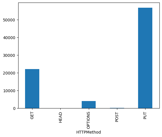

Now, we’re doing the string split on the whole dataframe. We could perform the manipulation /after/ we’ve filtered the data:

1
2
3

# Pandas plot() - filtering first
data_original["HTTPMethod"] = data_original.loc[data_original["vhost"].isin(["matrix.prof-x.net","matrix.prof-x.net:443", "matrix.prof-x.net:8448"])]["request"].str.split(" ").str[0]
data_original.groupby(["HTTPMethod"]).size().plot(kind='bar')

The result is:

97.1 ms ± 4.03 ms per loop (mean ± std. dev. of 5 runs, 5 loops each)

It doesn’t result in a much faster response because matrix.prof-x.net has 83108 rows of the 94046 rows. This means the str.split still has to do the majority of all the rows. If i take a much smaller result of the filter, then things are a lot faster because the str.split() has to do less rows. We also have to apply .copy() to avoid a python warning. So, in the end, filtering the data first and then str.split’ing will be faster, but on matrix.prof-x.net it’s not noticable. If the filter resulted in a much smaller dataframe, then it would be noticable.

Swifter

For swifter we can use the .swifter.apply() syntax to perform the string.split. We however bumped into an interesting problem at first. Some of the other hosts don’t have a normal request value. This likely has to do with how i parse the CSV file. It however shows that using For some other reason, a few of the rows inside the DataFrame store a float/NaN for the request value. I therefor had to write a little function to parse that correctly - which of course makde it a lot slower:

1
2
3

# Swifter - filter first
data_original["HTTPMethod"] = data_original.loc[data_original["vhost"].isin(["matrix.prof-x.net","matrix.prof-x.net:443", "matrix.prof-x.net:8448"])]["request"].swifter.apply(lambda x: x.split(" ")[0])
data_original.groupby(["HTTPMethod"]).size().plot(kind='bar')

The resulting graph looks the same. It did take a longer though:

174 ms ± 7.6 ms per loop (mean ± std. dev. of 5 runs, 5 loops each)

It was pointed out to me that swifter has a groupby option, i’m not using that here and thus this is not the most optimal solution.

Dask

Because Dask is lazy evaluation, it means that it’s really hard to compare /just/ the plotting part of the code. So, the example complete code would turn into:

 1
 2
 3
 4
 5
 6
 7
 8
 9
10
11
12
13
14
15

%%timeit -n 5 -r 5
# Dask read and plot
data_original = dd.read_csv('vhostcombined.log',
    sep=r'\s(?=(?:[^"]*"[^"]*")*[^"]*$)', engine='python', na_values='-', header=None, usecols=[0, 2, 4, 5, 7, 8, 9, 10, 11],
    names=['vhost', 'ip', 'user', 'time', 'request', 'status', 'size', 'referer', 'user_agent'],
    dtype={'user': object})

data_original["time"] = data_original["time"].apply(parse_datetime, meta=datetime)
data_original["request"] = data_original["request"].apply(parse_str, meta=str)
data_original["referer"] = data_original["referer"].apply(parse_str, meta=str)
data_original["user_agent"] = data_original["user_agent"].apply(parse_str, meta=str)


data_original["HTTPMethod"] = data_original.loc[data_original["vhost"].isin(["matrix.prof-x.net","matrix.prof-x.net:443", "matrix.prof-x.net:8448"])]["request"].apply(lambda x: x.split(" ")[0], meta=str)
data_original.groupby(["HTTPMethod"]).size().compute().plot(kind='bar')

This executes in:

2.14 s ± 128 ms per loop (mean ± std. dev. of 5 runs, 5 loops each)

This isn’t a bad result. If i change my pandas code to read and plot, it ends up being 2.09 seconds. The difference is very small again. We do need to point out that some people suggest to use hvplot in combination with dask. I guess that’s a whole other blogpost!

Polars

As mentioned, polars has a very different API. So, i had to rewrite the code quite a bit to get what i wanted:

1
2
3

# Polars filtering
filtered = data_original.filter(pl.col("vhost").is_in(["matrix.prof-x.net","matrix.prof-x.net:443", "matrix.prof-x.net:8448"]))
filtered.select(pl.col("*"), pl.col("request").apply(lambda x: x.split(" ")[0]).alias("HTTPMethod")).groupby(pl.col("HTTPMethod")).count().to_pandas().plot(kind='bar', x="HTTPMethod")

The result:

107 ms ± 14.9 ms per loop (mean ± std. dev. of 5 runs, 5 loops each)

That’s amazing! However, when i do the reading and plotting i end up on 2.22 seconds. This indicates (to me) that reading data and the from_pandas() call we have to do takes time, but the actual filtering and modifying of data does seem very fast.

Concluding

There’s a whole host of options here and they all have their benefits and downsides. In this specific case (reading a HTTP logfile) it’s a shame that we have to read data via pandas’s own read_csv to then convert it to a polars dataframe. Polars seems to be very efficient in querying the data.

This (to me) means that learning polars could be beneficial for performance in the long run.

The currrent set of data in this example is about 95.000 rows. That’s actually not so much. The results here could very massively with a much larger set of data.